Step-by-Step Guide: Spotlighting Maximum/Minimum Data Points in Excel Tables

Quick Links

• Apply a Quick Conditional Formatting Ranking Rule
• Create a Custom Conditional Formatting Ranking Rule

Automatically highlighting data in your spreadsheets makes reviewing your most useful data points a cinch. So if you want to view your top- or bottom-ranked values, conditional formatting in Microsoft Excel can make that data pop.

Maybe you use Excel to track your sales team’s numbers, your students’ grades, your store location sales, or your family of website’s traffic. You can make informed decisions by seeing which rank at the top of the group or which fall to the bottom. These are ideal cases in which to use conditional formatting to call out those rankings automatically.

Apply a Quick Conditional Formatting Ranking Rule

Excel offers a few ranking rules for conditional formatting that you can apply in just a couple of clicks. These include highlighting cells that rank in the top or bottom 10% or the top or bottom 10 items.

Select the cells that you want to apply the formatting to by clicking and dragging through them. Then, go to the Home tab and over to the Styles section of the ribbon.

Click “Conditional Formatting” and move your cursor to “Top/Bottom Rules.” You’ll see the above-mentioned four rules at the top of the pop-out menu. Select the one that you want to use. For this example, we’ll choose the Top 10 Items.

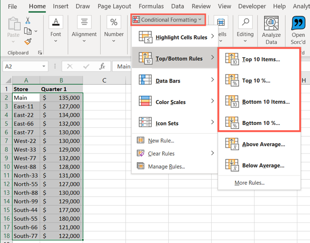
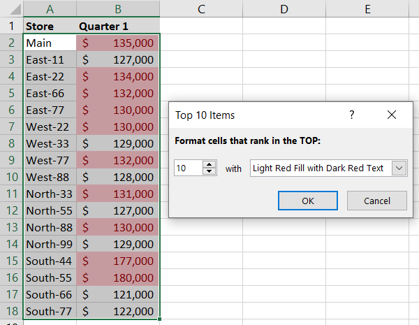
Excel immediately applies the default number (10) and formatting (light red fill with dark red text). However, you can change either or both of these defaults in the pop-up window that appears.

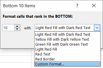
On the left, use the arrows or type in a number if you want something other than 10. On the right, use the drop-down list to choose a different format.

Click “OK” when you finish, and the formatting will be applied.

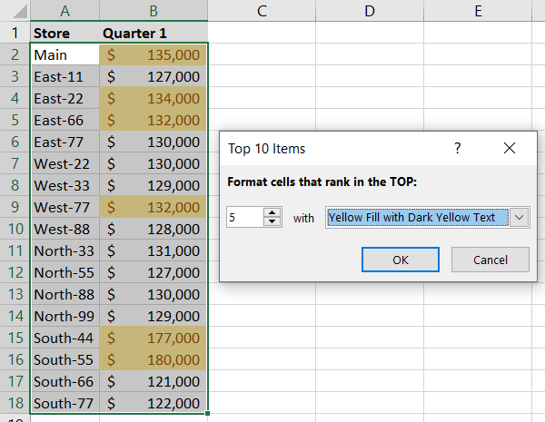
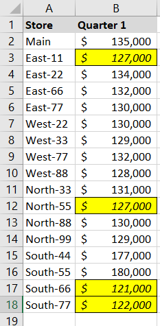
Here, you can see that we’re highlighting the top five items in yellow. Since two cells (B5 and B9) contain the same value, both are highlighted.

With any of these four quick rules, you can adjust the number, percentage, and formatting as needed.

Create a Custom Conditional Formatting Ranking Rule

While the built-in ranking rules are handy, you might want to go a step further with your formatting. One way to do this is to select “Custom Format” in the above drop-down list to open the Format Cells window.

Another way is to use the New Rule feature. Select the cells that you want to format, head to the Home tab, and click “Conditional Formatting.” This time, choose “New Rule.”

When the New Formatting Rule window opens, select “Format Only Top or Bottom Ranked Values” from the rule types.

Easy and Safe Partition Software & Hard Disk Manager

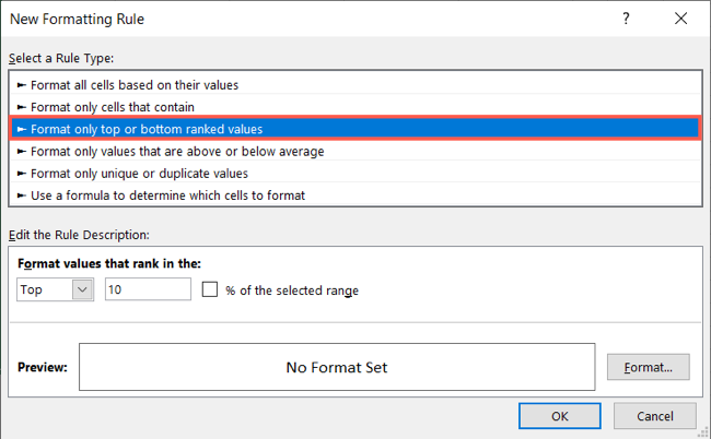
At the bottom of the window is a section for Edit the Rule Description. This is where you’ll set up your number or percentage and then select the formatting.

In the first drop-down list, pick either Top or Bottom. In the next box, enter the number that you want to use. If you want to use percentage, mark the checkbox to the right. For this example, we want to highlight the bottom 25%.

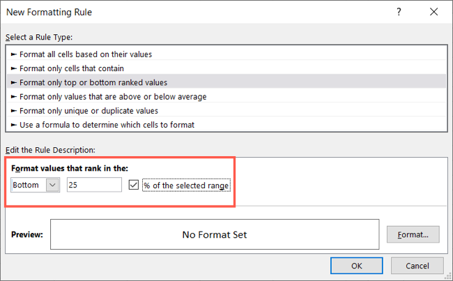
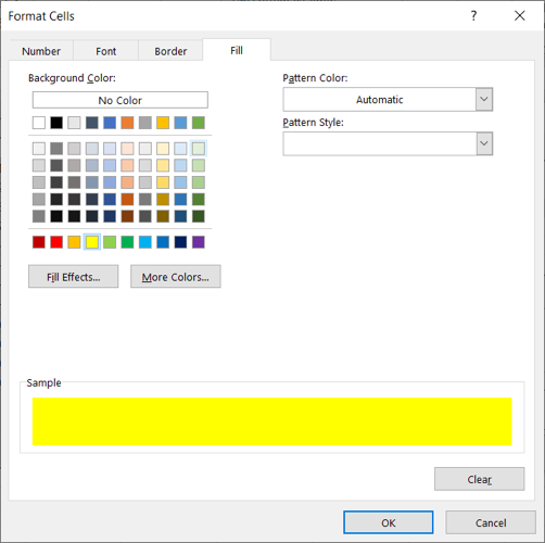
Click “Format” to open the Format Cells window. Then, use the tabs at the top to choose Font, Border, or Fill formatting. You can apply more than one format if you like. Here, we’ll use an italic font, a dark cell border, and a yellow fill color.

Click “OK” and check out the preview of how your cells will appear. If you’re good, click “OK” to apply the rule.

SwifDoo PDF 2-Year Plan

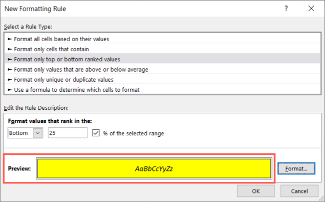
You’ll then see your cells immediately update with the formatting that you selected for the top- or bottom-ranked items. Again, for our example, we have the bottom 25%.

If you’re interested in trying out other conditional formatting rules, take a look at how to create progress bars in Microsoft Excel using the handy feature!