Step-by-Step Guide: Combining Two Excel Columns Efficiently

Quick Links

Some tasks for taking care of data in Excel are intuitive, like inserting currency . Then there are others that are not, like combining columns. We’ll show you a few different ways to merge two columns in Microsoft Excel.

You may have imported data from an external location or had someone enter data in your sheet . If you end up with two columns that would work better as one, you can combine them using an operator or a function .

About Merging Columns in Excel

As you may know, Excel has a Merge Cells feature. Unfortunately, when you use this option, only the data in the first (far-left) cell is retained. So if you want to combine two columns and keep all data intact, this is not a feature you want to use.

To hold onto the data in two columns, you’ll merge all data into a third column. Before you begin combining the data in the cells as described below, you should prepare by inserting another column if necessary.

You’ll then perform the following steps:

Merge two cells, one from each column, in the first row.
Copy the formula to the remaining rows in the merged column.
Optional: Convert the formulas to static values.

Merge Cells in Columns

You have two ways to initially merge cells before copying their contents: using an ampersand operator or using the CONCAT function. We’ll cover both.

Method 1: Using the Ampersand Operator

The ampersand symbol (&) has more uses than a shorter way to type the word “and.” You can use the ampersand operator in a formula to combine data in cells.

Go to the cell in the first row of your new column for the merged data and insert one of the following formulas replacing the cell references with your own.

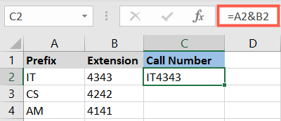
To merge the cells A2 and B2, you would enter the following formula and press Enter:

=A2&B2

This combines the data in those two cells into one string.

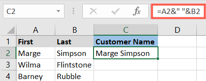
To merge the cells A2 and B2 with a space in the middle, you would use the following formula:

=A2&” “&B2

Note the space between the parentheses. This is handy for combining first and last names or words that need a space between.

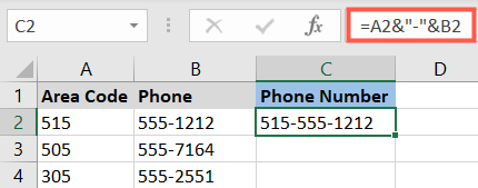
To merge the cells in A2 and B2 with a hyphen in the middle, you would use this formula:

=A2&”-“&B2

This is convenient for merging phone numbers or product identifiers.

After this, you can move on to the next step , copying the formula.

Method 2: Using the CONCAT Function

While merging cells and columns with the ampersand operator isn’t difficult, it does require some extra typing. Instead, you can use the CONCAT function or the older CONCATENATE function .

Go to the cell in the first row of your new column for the combined data and use one of the following formulas. Remember to replace the cell references with your own.

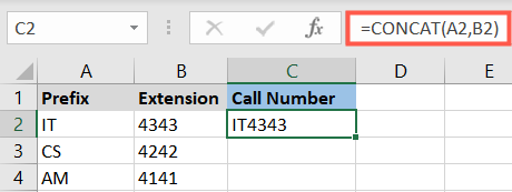
To merge the cells A2 and B2, you would enter the following formula and press Enter:

=CONCAT(A2,B2)

The result is the same as the first ampersand formula above. You have one string without spaces.

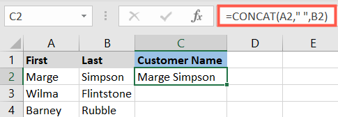
To merge the cells A2 and B2 with a space in the middle, you would use the following formula:

=CONCAT(A2,” “,B2)

With this formula, you can place a space between text or numbers. Note the space between the parentheses.

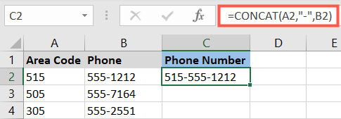
To merge the cells in A2 and B2 with a hyphen in the middle, you would use this formula:

=CONCAT(A2,”-“,B2)

Again, this is useful for numbers or even words that contain dashes.

Now that you’ve merged two cells in a row of your two columns, it’s time to copy the formula.

Copy the Formula

Once you have the first formula inserted, you don’t have to enter it manually for each row in your column. Simply copy the formula down.

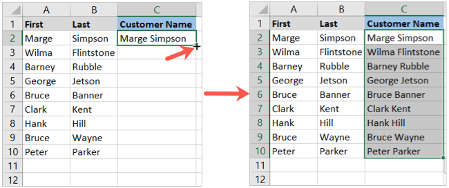
Select the cell containing the formula. When the Fill Handle (plus sign) appears on the bottom right corner of the cell border, double-click. This copies the formula as far down the column as there is data, which is ideal for columns that span many, many rows.

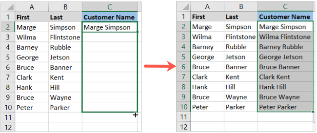
Alternatively, you can drag the plus sign as far as you need to, rather than double-clicking it. You might use this option if you want to stop at a certain point in the column.

Optional: Convert the Formulas

One final step you may want to take is to convert the formulas to static values. If you plan to delete the original columns and keep only the merged column, you must convert the data first. This is because the formulas use the cell references in those columns to combine the data. So, if those cell references no longer contain the data, you won’t have the merged data.

If this is a step you’re interested in, take a look at our full tutorial for converting formulas to static data in Excel .

Win Dash

Step-by-Step Guide: Combining Two Excel Columns Efficiently