Mastering Excel: Effective Strategies for Concealing Comments, Formulas, Excess Text & Gridlines

Quick Links

We’ve shown you how to hide cells, rows, and columns and how to hide worksheets/tabs and entire workbooks in Excel. Additionally, you can hide items such as comments, formulas, overflow text, and gridlines. We’ll show you how to hide these items.

Hide Comments

When you add a comment to a cell in Excel, a small red triangle displays in the upper-right corner of the cell to indicate a comment was added. When you hover your mouse over the cell, or select the cell, the comment displays in a popup window.

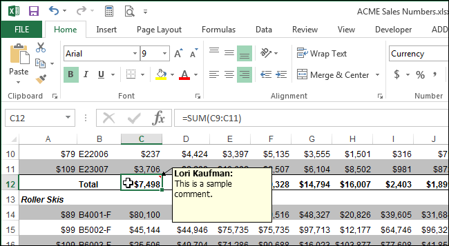
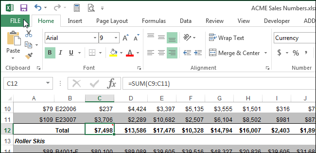
If you have a lot of comments in your worksheet, you may not want to see the red triangles and have comments popup as you move your mouse around the worksheet. To hide the comments, click the “File” tab.

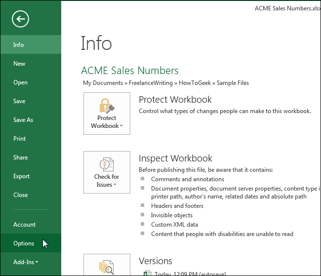
On the backstage screen, click “Options” in the list of items on the left.

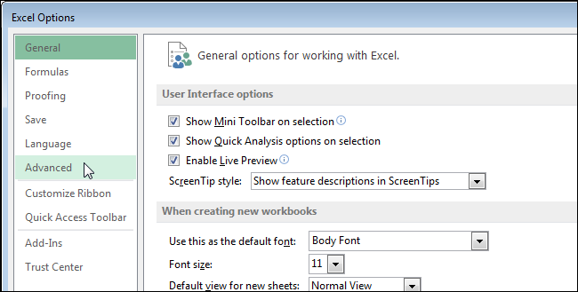
On the “Excel Options” dialog box, click “Advanced” in the list of items on the left.

Scroll down to the “Display” section. Under “For cells with comments, show”, select the “No comments or indicators” radio button.

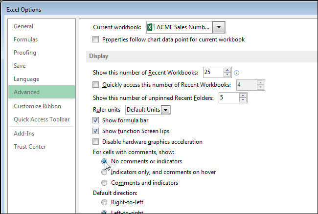
Click “OK” to accept the change and close the “Excel Options” dialog box.

The red triangles and comment popup windows are now hidden.

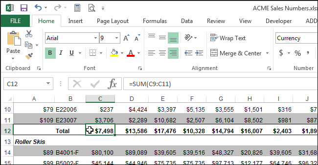
The comments are still associated with their respective cells and can be viewed by clicking the “Review” tab and clicking “Show All Comments” in the “Comments” section.

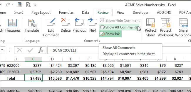
All the comments in your worksheet are displayed without having to hover over the cells. To hide the comment popup windows, click “Show All Comments” again. The comment popup windows are hidden but the red triangles remain visible.

NOTE: If you want to show or hide a comment for a certain cell, select that cell and click “Show/Hide Comment” in the “Comments” section of the “Review” tab. You can select multiple cells with comments using the “Ctrl” key to show or hide the comments on those cells only.

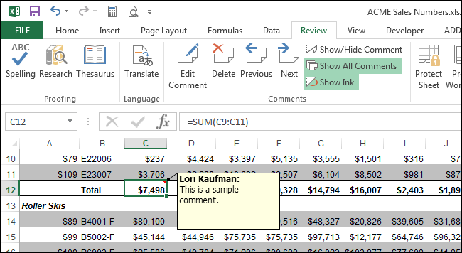
Clicking the “Show All Comments” button so it toggles off changes the “For cells with comments, show” option back to “Indicators only, and comments on hover” automatically.

Hide Formulas

There are two things you need to do to hide a formula. First, you must apply the “Hidden” setting to the cell and then protect the worksheeet.

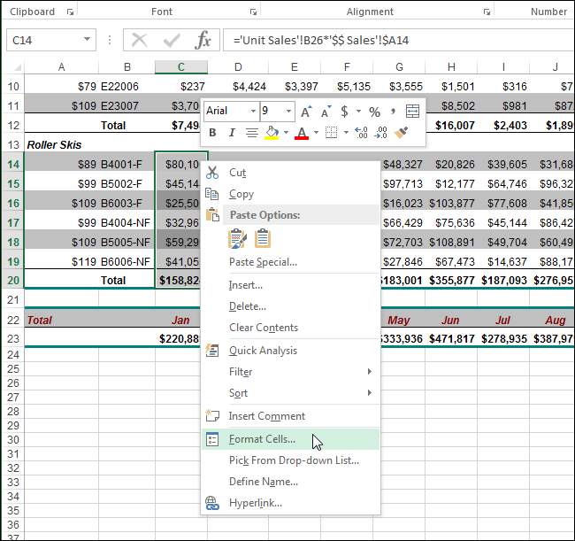
Select the cell for which you want to hide the formula and right-click on the selected cell. Select “Format Cells” from the popup menu.

NOTE: You can select multiple cells and hide the formulas for all the selected cells.

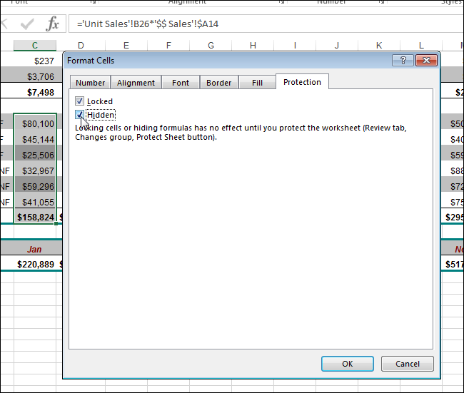
Click the “Protection” tab on the “Format Cells” dialog box, and select the “Hidden” check box so there is a check mark in the box. Click “OK” to accept the change and close the dialog box.

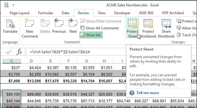
The formulas won’t be hidden until you protect the sheet. To do this, click the “Review” tab and click “Protect Sheet” in the “Changes” section.

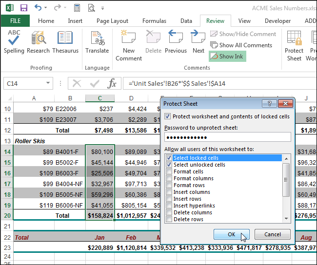
The “Protect Sheet” dialog box displays. To prevent other users from unhiding the formulas, enter a password in the “Password to unprotect sheet” edit box. Specify the actions you want to allow users to perform on the worksheet by selecting check boxes in the “Allow all users of this worksheet to” list. Click “OK” to accept your changes and close the dialog box.

NOTE: The password is not required, but we recommend you enter one if you don’t want other users to be able to unprotect the worksheet.

A dialog box displays asking you to confirm your password.

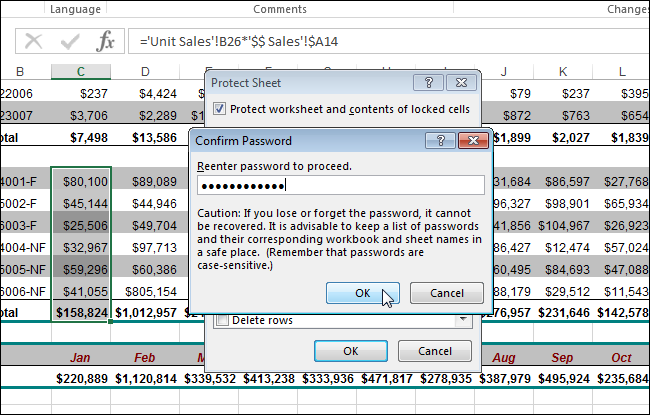
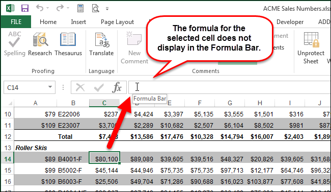
The formulas in the selected cells do not display in the Formula Bar, but the results of the formulas remain visible in the cells. If you entered a password when protecting the sheet, other users will not be able to use the “Show Formulas” button on the “Formulas” tab to display all the formulas in the worksheet.

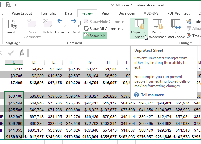
To unhide the formulas, click “Unprotect Sheet” in the “Changes” section of the “Review” tab.

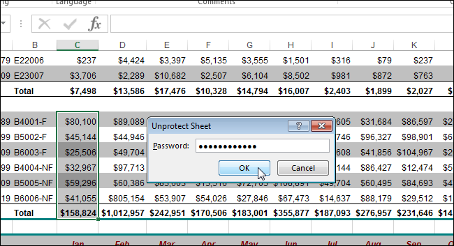
If you entered a password when protecting the sheet, the “Unprotect Sheet” dialog box displays, prompting you for the password. Enter the password in the “Password” edit box and click “OK”. If you didn’t enter a password when protecting the sheet, the sheet will be unprotected with no further prompts.

Select the cells for which you hid the formulas, right-click on the cells, and select “Format Cells” from the popup menu. Deselect the “Hidden” option on the “Protection” tab of the “Format Cells” dialog box so there is NO check mark in the box.

Another way to hide formulas from other users is to convert the formulas to static values and save the workbook with a different filename. Then, distribute this new workbook to the users.

Click here

Hide Overflow Text

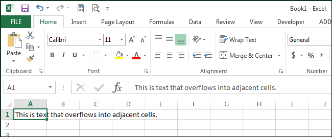
When you type a lot of text into a cell in Excel, it overflows over to the adjacent cells. For example, the text entered into cell A1 in the image below overflows into cells B1 through E1.

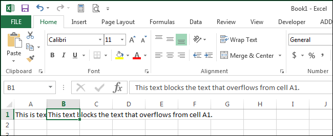
If we type text into cell B1, the overflow text from cell A1 is blocked by the text in cell B1.

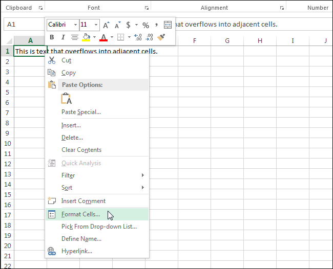
If you want to hide the overflow text in a cell, such as A1 in this example, without having to type anything into the adjacent cells, right-click on the cell and select “Format Cells” from the popup menu.

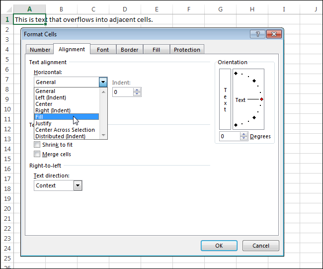
On the “Format Cells” dialog box, click the “Alignment” tab. Select “Fill” from the “Horizontal” drop-down list. Click “OK” to accept the change and close the dialog box.

The overflow text from cell A1 is hidden even though there is no text in cell B1.

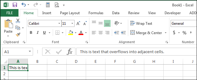
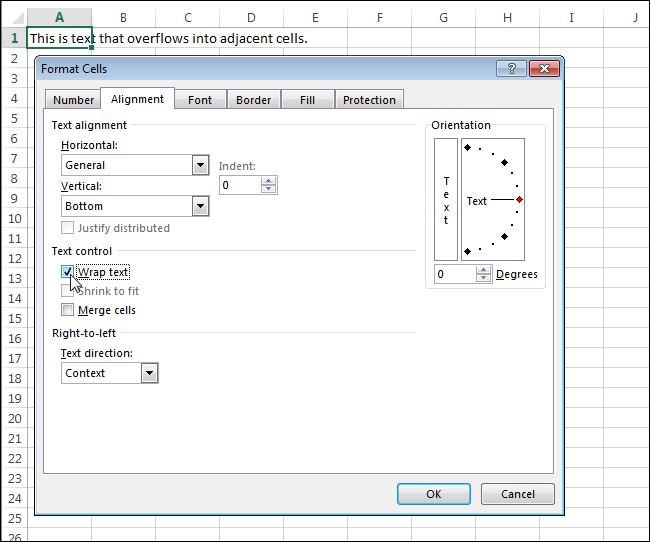
You can prevent text from overflowing to adjacent cells using the “Wrap Text” feature. Select the cell containing overflowing text and access the “Format Cells” dialog box as described earlier in this article. Click the “Alignment” tab and select the “Wrap text” check box so there is a check mark in the box. Click “OK” to accept the change and close the dialog box.

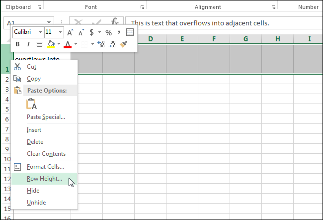
When you choose to wrap text in a cell, the cell height is adjusted to accommodate the text. If you want to keep the row height at the standard value (15) for a single line of text, right-click on the row number and select “Row Height” from the popup menu.

On the “Row Height” dialog box, type “15” in the edit box and click “OK”.

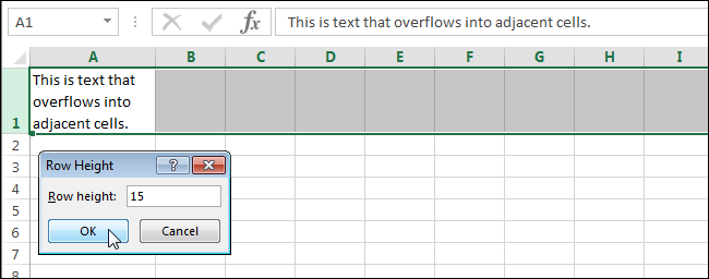
The row height is adjusted and the remaining text that doesn’t fit on the first line appears to be hidden.

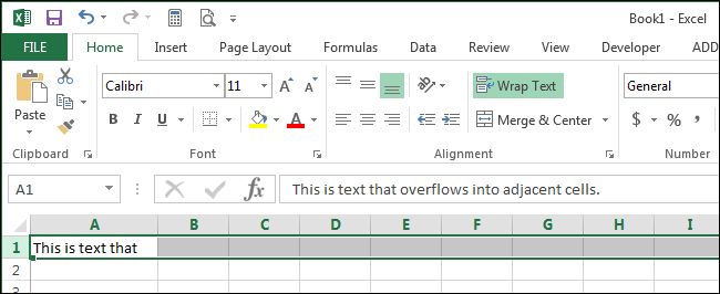
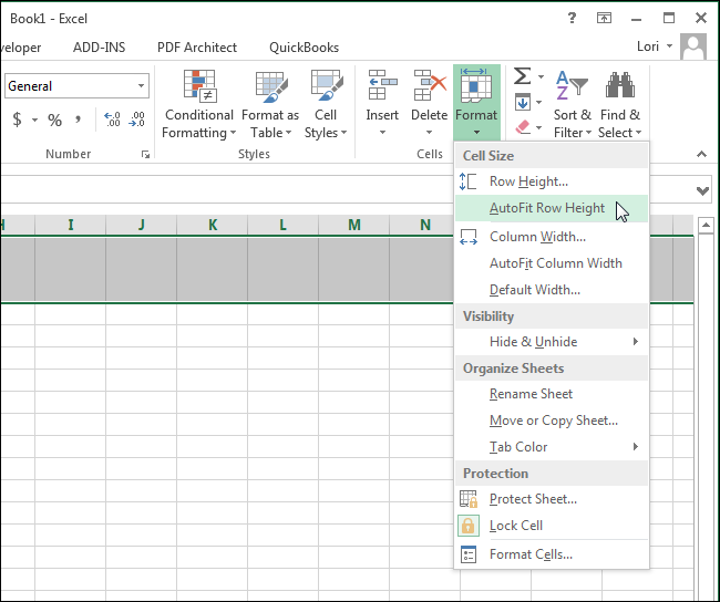
If you don’t change the “Row Height” back to its original value and you turn off the “Wrap text” feature, you’ll notice that the text now takes up only one line but the height of the row remains the same as it was when it adjusted to accommodate the wrapped text. You can either set the “Row Height” to “15” or you can automatically adjust the row height to fit the one line of text using the “AutoFit Row Height” feature. Make sure the “Home” tab is the active tab on the ribbon and click “Format” in the “Cells” section. Select “AutoFit Row Height” in the “Cell Size” section on the drop-down menu.

Hide Gridlines

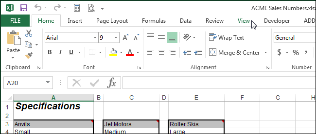
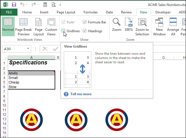
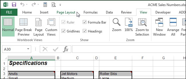
If you are displaying your worksheet in a presentation, you can hide the gridlines to make the presentation of the data in your worksheet cleaner. There are a couple of different methods you can use to hide all the gridlines in a worksheet. For the first method, click the “View” tab.

Select the “Gridlines” check box in the “Show” section so there is NO check mark in the box.

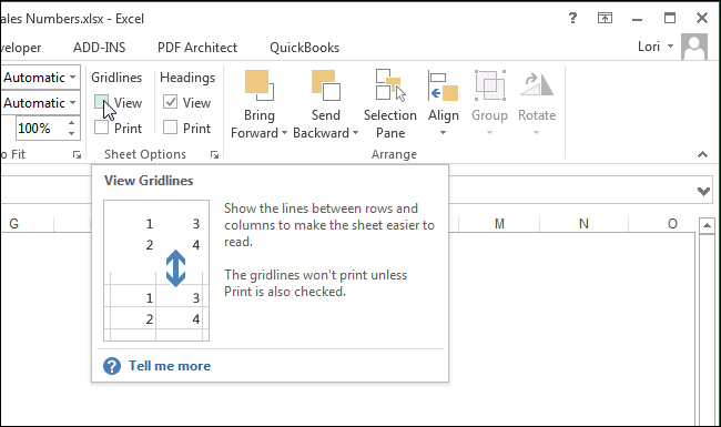
For the second method, click the “Page Layout” tab.

Under “Gridlines” in the “Sheet Options” section, select the “View” check box so there is NO check mark in the box.

Remember, you can also hide other items in Excel such as cells, rows, and columns and worksheets/tabs and even entire workbooks .

Win Dash

Mastering Excel: Effective Strategies for Concealing Comments, Formulas, Excess Text & Gridlines