How to Manage Excel Bookmark Alternatives: A Clever Hack You Need

Quick Links

Do you have a massive Excel workbook containing lots of worksheets with many rows and columns? Do you find yourself endlessly scrolling or jumping from one tab to the other? Stop there, because this hack will resolve this issue for you.

What is a Bookmark (in Word)?

A bookmark is an invisible way-point in a Word document (don’t worry—we’ll get to the Excel bit shortly). To set one, with your cursor at the point you want to mark, go to the “Insert” tab on the ribbon and click “Bookmarks” in the “Links” group. Here, you can give your bookmark a name (with no spaces).

You can add or link to as many bookmarks as you wish in a document, and they are really useful if, for example, you want to mark and jump to an important location in your document. Doing this can also be handy to save time if you’d otherwise have to scroll through a long document, where you could also miss what you’re looking for. It’s also great for creating hyperlinks to certain parts of your work.

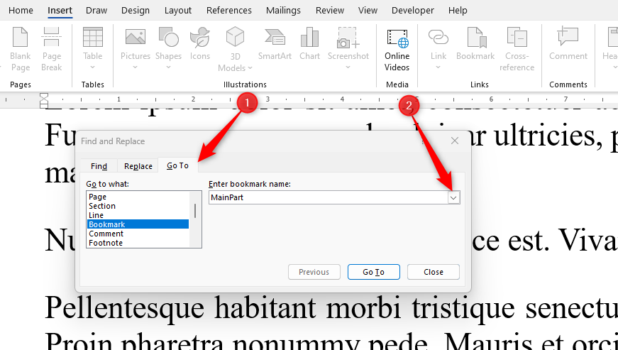
To jump to a bookmark you’ve set in Word, press Ctrl+G (or Ctrl+Cmd+G on a Mac), open the “Go To” tab, click “Bookmark”, and use the drop-down to choose where you want to go.

However, to do the same thing (and more) in an Excel workbook, you have to take a different route.

How to Set and Locate a Bookmark (Name) in Excel

In Excel, bookmarks are called—somewhat unimaginatively—names, accessible through the name box in the top-left corner of your workbook. In fact, every cell already has its own bookmark, or name, which you can see by selecting any cell and looking at the name box.

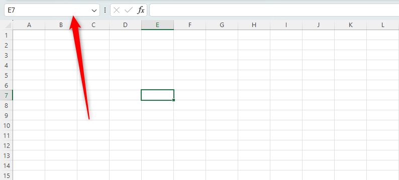
To jump to a cell within the active worksheet—useful if you have hundreds of rows or columns within that sheet—type the column-row reference, such as E7, into the name box and press Enter. If you have other active tabs in your workbook, you can jump to any cell within any of the worksheets by typing the tab name, followed by an exclamation mark, and then the cell reference. For example,

Sheet2!G5

would take us to Sheet 2, cell G5. Or you can type just the tab name, which would take you to an unspecified location within that sheet.

You can also use the name box to highlight a range of cells. For example, if you were to type

E1:P42

in the name box, this would highlight these cells for you in the current sheet, handy if you want to select a large range of cells. Try this out with other combinations, such as

R:R

to highlight the whole of column R, or

5:5

to highlight the whole of row 5.

While cells already have their own reference names, you can change what they’re called by selecting the cell and typing a new name in the name box. What’s more, you can also name a range of data. Let’s say you have an important data range in your large workbook that you need to view often. Simply select the data and give it a name.

You’ll need to use a slightly different method to name a formatted table. Go to the bottom of this section for instructions on how to do this.

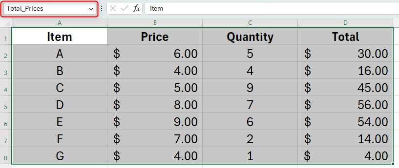
Excel doesn’t like spaces in names. If you want to use more than one word in the name, either type them without a space (for example, TotalPrices), or use an underscore (Total_Prices).

You can also name other elements in your workbook—such as charts or illustrations—in the same way. Unfortunately, you can only use the name box to jump to a cell or range of cells (you can’t jump to charts or illustrations), but naming a chart can be useful in VBA coding .

No matter where you are in your workbook, click the drop-down arrow next to the name box and instantly jump to the cells you’ve named.

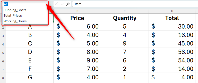
If you prefer to use keyboard shortcuts, press F5 to bring up the Go To dialog box.

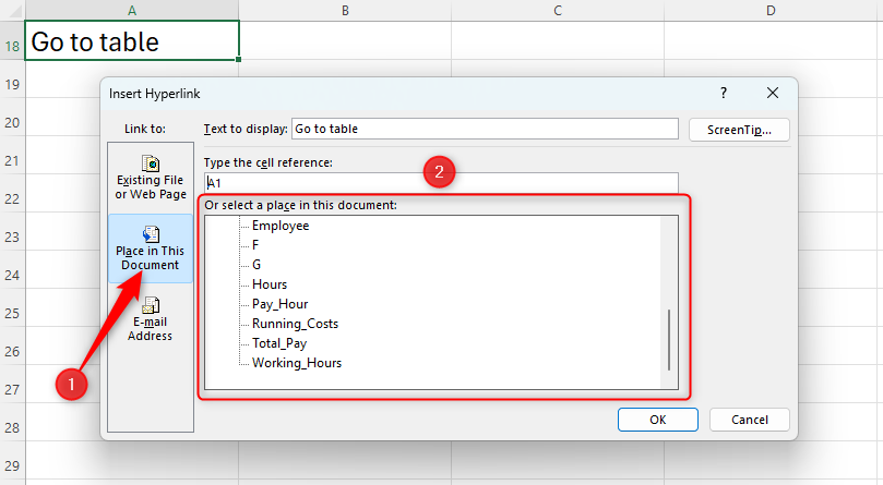
You can also create a hyperlink to named cells in your workbook. Right-click the cell where you want the hyperlink to go, and choose “Link” from the options that appear. Then, click “Place In This Document”, choose the name you want to link to, and click “OK.”

Click here

Naming a Formatted Table (It’s Slightly Different)

If you use a table within your workbook, we recommend that you format it properly using Excel’s built-in table formatter . Then, if you add additional columns or rows to your table, the name you have given to your array will extend to include the new data. Importantly, after formatting your table, you need to use a different name box, which means you’ll be able to reference the table in formulas later on. We will discuss this more in the final section of this article.

Select any cell within your table, and click the “Table Design” tab on the ribbon. Head to the Properties group and change the name of your table, before pressing Enter.

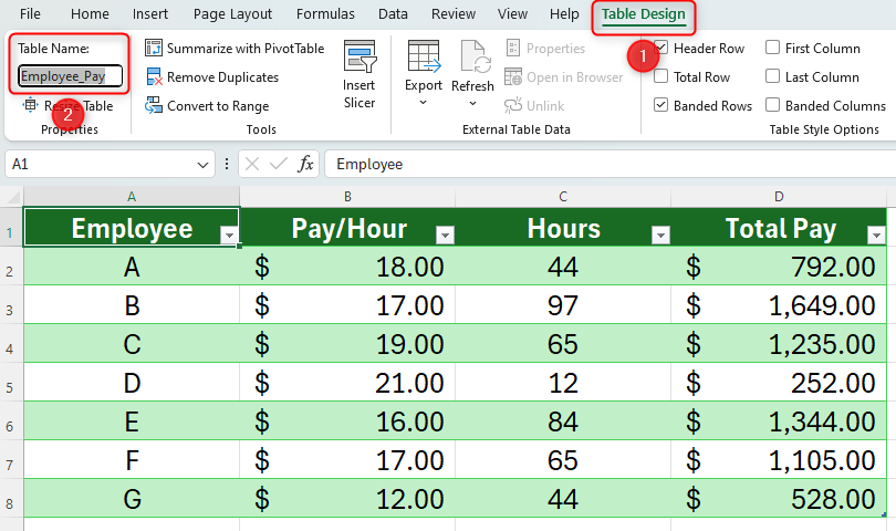
You will now see the name of the table appear when you click the drop-down arrow next to the name box. Even though you used a different method to name your table, your table appears as a named array in the usual way.

How to Remove or Edit Names in Excel

You might accidentally create a name for a cell or range when you actually meant to jump to a certain item. Or, maybe, you need to change a name you’ve already assigned. To remove or change names in Excel, in the Formulas tab on the ribbon, click “Name Manager” in the Defined Names group. You can also create a new bookmark in the window that appears, but it’s definitely easier to do this on the worksheet itself using the methods outlined above.

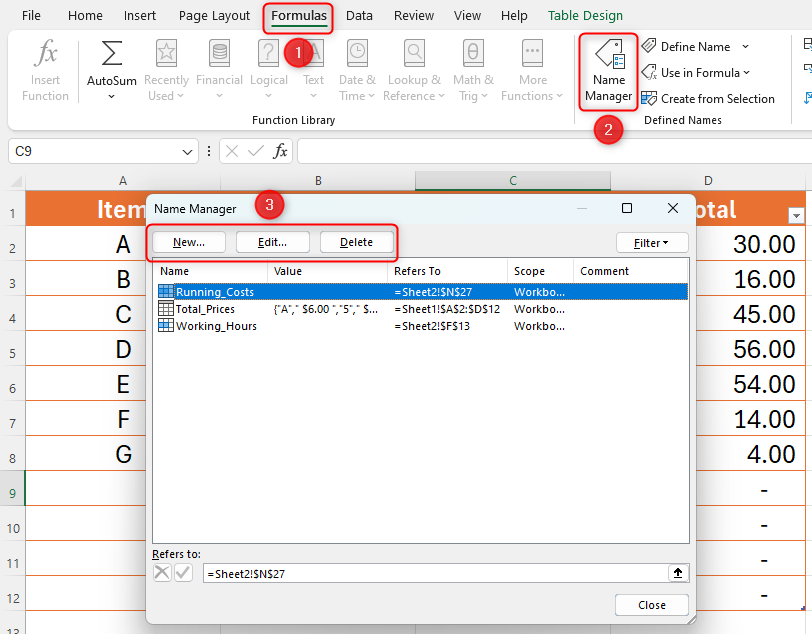
When you’re done managing the names in your workbook, click “Close” in the bottom right-hand corner of the window.

Click here

Other Reasons for Using the Name Box

Now that you’ve assigned names to cells within your workbook, let’s look at other name box gems.

Reference a Name Within a formula

In the example below, we have an accounting table on a separate tab in our workbook, and want to pull data from our table on Sheet 1. Because we’ve named our data range, we can use that name within a formula, and Excel will help us to do that.

Start by typing the calculation you want to create. In our case, we want to sum the employees’ pay.

=sum(

Now, begin typing the name of the data range. In our case, it’s Employee_Pay.

=sum(em

You’ll notice that the name you have given the data range appears.

Double-click the data name.

We now want to tell Excel to use the Total Pay column within our table, and we do this by opening a square parenthesis.

=sum(Employee_Pay[

This time, Excel will bring up each column name within your named table.

Double-click the column name, close the square parenthesis, and close the formula parenthesis, before pressing Enter.

=sum(Employee_Pay[Total Pay])

This will successfully sum all values in that column, and will also pick up changes or additions to the values in the column because you’ve named the table. We would then go ahead and use the same technique to complete the other totals and averages in our accounting table.

Create Names for Columns in Tables

Finally, if you have a large table of data, you might want to create a bookmark for an important row or column that you want to access quickly.

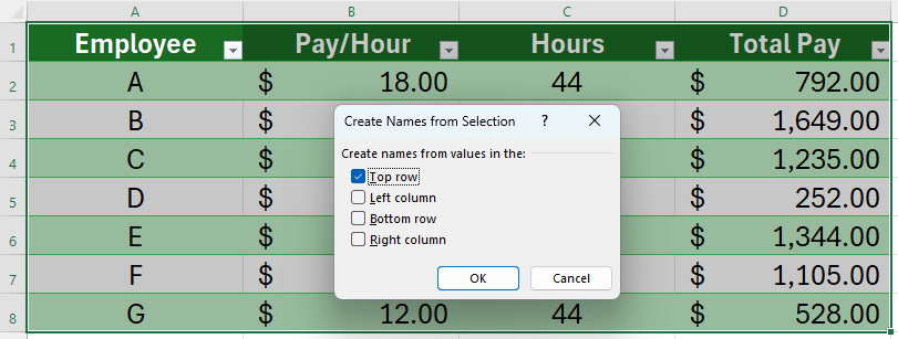
Highlight your table, and in the “Formulas” tab on the ribbon, click “Create From Selection”.

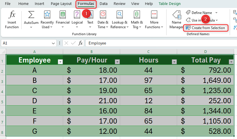
You can then choose which names you want to create and click “OK.” In our example, if we choose “Top Row,” this will result in the column names being added to the name list for easier access later on.

If you have a particularly large spreadsheet, you may not remember which names refer to which ranges. In this case, you can generate a list of names and their associated cell ranges you can reference as you type your formulas for that spreadsheet.

Win Dash

How to Manage Excel Bookmark Alternatives: A Clever Hack You Need