Formatting Positive and Negative Data in Microsoft Excel Easily Explained

Quick Links

Microsoft Excel displays negative numbers with a leading minus sign by default. It is good practice to make negative numbers easy to identify, and if you’re not content with this default, Excel provides a few different options for formatting negative numbers.

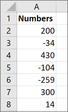
Excel provides a couple of built-in ways to display negative numbers, and you can also set up custom formatting. Let’s dive in.

Change to a Different Built-In Negative Number Option

One thing to note here is that Excel will display different built-in options depending on the region and language settings in your operating system.

For those in the US, Excel provides the following built-in options for displaying negative numbers:

In black, with a preceding minus sign
In red
In parentheses (you can choose red or black)

In the UK and many other European countries, you’ll typically be able to set negative numbers to show in black or red and with or without a minus sign (in both colors) but have no option for parentheses. You can learn more about these regional settings on Microsoft’s website .

No matter where you are, though, you’ll be able to add in additional options by customizing the number format, which we’ll cover in the next section.

To change to a different built-in format, right-click a cell (or range of selected cells) and then click the “Format Cells” command. You can also press Ctrl+1.

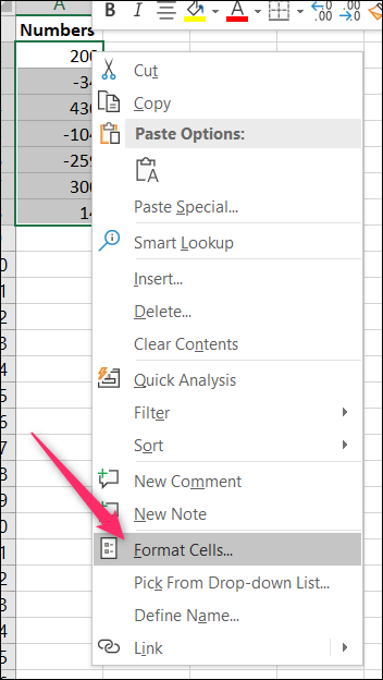
In the Format Cells window, switch to the “Number” tab. On the left, choose the “Number” category. On the right, choose an option from the “Negative Numbers” list and then hit “OK.”

Note that the image below shows the options you’d see in the US. We will be talking about creating your own custom formats in the next section, so it’s no problem if what you want is not shown.

Click here

Here, we’ve chosen to display negative values in red with parentheses.

This display is much more identifiable than the Excel default.

Create a Custom Negative Number Format

You can also create your own number formats in Excel. This provides you with the ultimate control over how the data is displayed.

Start by right-clicking a cell (or range of selected cells) and then clicking the “Format Cells” command. You can also press Ctrl+1.

On the “Number” tab, select the “Custom” category on the left.

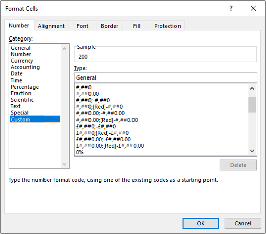
You’ll see a list of different custom formats on the right. This can seem a little confusing at first but is nothing to fear.

Each custom format is split into up to four sections, with each section separated by a semi-colon.

The first section is for positive values, the second for negatives, the third for zero values, and the last section for text. You do not have to have all sections in a format.

Click here

As an example, let’s create a negative number format which includes all of the below.

In blue
In parentheses
No decimal places

In the Type box, enter the code below.

#,##0;Blue

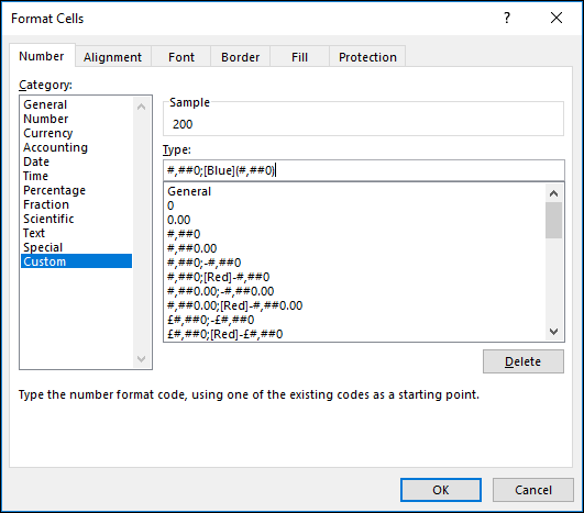
Each symbol has a meaning, and in this format, the # represents the display of a significant digit, and the 0 is the display of an insignificant digit. This negative number is enclosed in parenthesis and also displayed in blue. There are 57 different colors you can specify by name or number in a custom number format rule. Remember that the semi-colon separates the positive and negative number display.

And here’s our result:

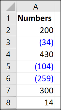
Custom formatting is a useful Excel skill to have. You can take formatting beyond the standard settings provided in Excel that may not be sufficient for your needs. Formatting negative numbers is one of the most common uses of this tool.

Win Dash

Formatting Positive and Negative Data in Microsoft Excel Easily Explained