Excel Mastery: Easily Identifying the Lowest and Highest Figures Using Simple Formulas

Quick Links

• Use the SMALL Function
• Use the LARGE Function
• A Limitation to Note

Key Takeaways

Use the SMALL function to find the smallest number and the LARGE function to find the largest number. Use either Excel function in the form =SMALL(range,position) or =LARGE(range,position). For example, =SMALL(B2:E13,1) will find the first smallest number in the range of cells between B2 and E13.

When you have a spreadsheet packed with data, finding the number you need can be tedious. Yet, whether you’re looking for the lowest product sales amount or the highest test score, Excel’s SMALL and LARGE functions can help.

Using these two Excel functions, you aren’t limited to only finding the smallest or largest number in a cell range. You can also locate the second smallest, third smallest, or fifth largest. For a quick way to find the number you want, here’s how to use the SMALL and LARGE functions in Excel .

Use the SMALL Function

The syntax for the function is

    `SMALL(range, position)`

where both arguments are required. You’ll enter the range or array for the

    `range`

argument. For the

    `position`

argument, enter a one for the first smallest number, two for the second smallest number, three for the third, and so on.

As an example, we’ll locate the smallest number in our cell range B2 through E13 using this formula:

=SMALL(B2:E13,1)

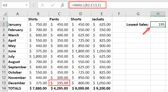
As another example, we’ll find the second smallest number in that same cell range. Here’s the formula:

=SMALL(B2:E13,2)

Use the LARGE Function

The LARGE function works the same way as the SMALL function, only providing you with the biggest number. The syntax is LARGE(range, position) with both arguments required and representing the same data as the SMALL function.

To find the largest number in our cell range B2 through E13, we’ll use this formula:

=LARGE(B2:E13,1)

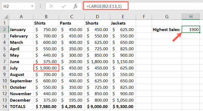
To locate the third largest number in that same cell range, we can use this formula:

=LARGE(B2:E13,3)

A Limitation to Note

It’s important to note a specific limitation when you use these functions. If you have duplicate numbers in your data, your result is skewed when finding different positions. Here’s an example.

Related: How to Highlight Duplicates in Microsoft Excel

Below, we searched for the largest number in our cell range B2 through E13. The result is 1,800, which is correct.

But, if we look for the second largest number in that same cell range, our result is also 1,800. This is because 1,800 appears twice, making it both the largest and second largest number.

Consider this limitation when searching for various positions in your cell range.

If you want to quickly find the lowest five sales totals in your product sheet or the highest three monthly bills in your budget , keep the SMALL and LARGE functions in mind.

For more, learn how to use INDEX and MATCH to find specific values or how to find range in Excel .

Also read: